#12 The Physics of: Crop Yield using physical crop growth models and weather data

In last week’s post we covered how soil moisture is monitored at field scale using an empirical relationship between Evaporative Fraction and Soil Moisture.

Soil moisture monitoring is desirable because it allows us to maintain moisture between a soil’s wilting point and field capacity and therefore maximize Crop Yield (tonnes/ha). Crop yield thus is an important outcome variable. Can we similarly use remote-sensing to track field scale crop yield operationally? This problem statement has attracted much attention from various angles, with physics based, statistical, machine learning and deep learning approaches used to tackle the challenge.
Method
In this post we’ll take a look at Scalable Crop Yield Mapper , a hybrid method (physical + statistical) for crop yield modeling developed and made popular by D. Lobell at Stanford. This method uses as a base physiological crop models, in particular the Agricultural Production Systems Simulator (APSIM).
The Agricultural Crop Production Model
In plainspeak, APSIM can simulate the growth of a plant, given local climate data (rainfall, temperature, humidity etc), typical local soil parameters (soil water content, nutrient levels etc) and crop management practices (sowing date, sowing density etc). The output of the model is simulated values of crop yield (tonnes/ha) and Leaf Area Index (LAI).
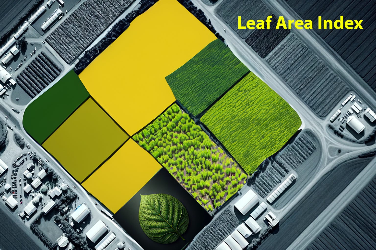
Leaf Area Index
The Leaf Area Index is an important concept in agricultural sciences which is a measure of leaf density per unit ground area. LAI is important because it is a quantifiable variable which is both a result of and directly influences a plant’s interaction with it’s environment. All else constant, a field with higher LAI absorbs more of the sun’s incident energy and transpires more water back to the environment. Higher LAI also is a proxy for higher crop yields.
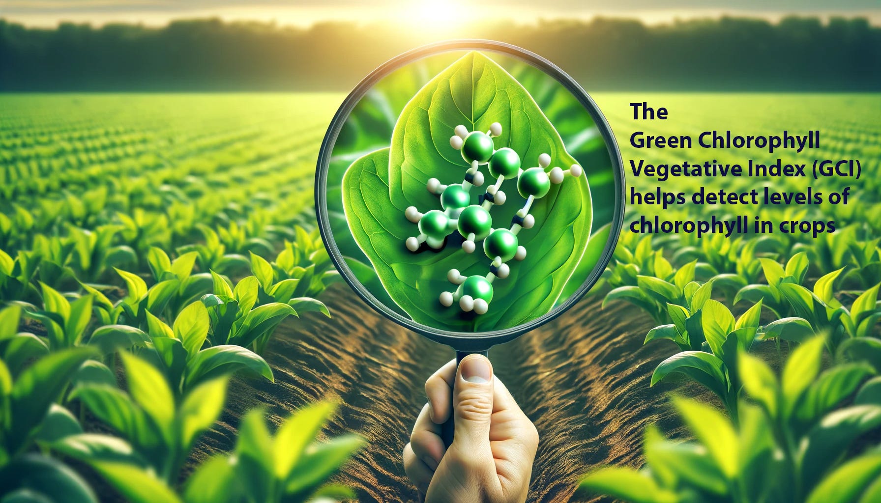
Green Chlorophyll Vegetative Index
Earth Observation satellites produce imagery that specifies how much each wavelength of light is reflected at each pixel. Green and Near Infrared are two wavelengths of light captured by most satellites, high green reflectance means more chlorophyll and hence more photosynthetic activity, high NIR reflectance is a proxy for more plant biomass. Combining these two, remote sensing scientists have developed the Green Chlorophyll Vegetative Index (GCVI) to represent plant health with common multispectral RS imagery. GCVI is easily measured using the formula below.
While Leaf Area Index is a useful concept for physiological models of crop growth, it is hard to accurately and directly observe LAI from remote sensing data. Multiple studies have established relationships between LAI and Vegetative Indices (e.g. GCVI) for different crops which can be directly observed from remote sensing imagery.
Thus the simulated LAI values can be turned into corresponding simulated GCVI values. Practically, this means that we have a prior expectation based on a physical crop model for what Yield and GCVI we can expect to see for a given set of cropping practices, soil and input data.
Yield vs GCVI
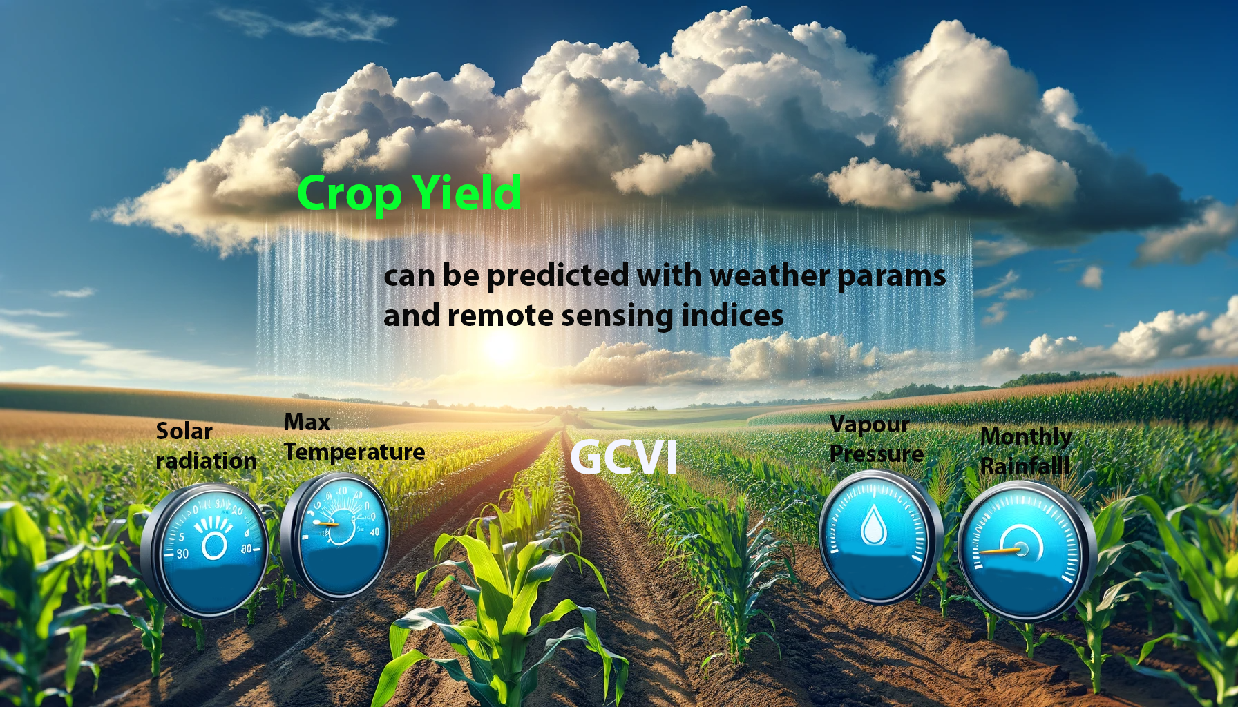
Using the simulated values of GCVI we now only need to establish a relationship between Yield and GCVI. With this relationship we can operationally monitor Crop Yield based on regularly produced GCVI from satellite imagery. The SCYM method takes the simulated crop yield values and with a simple multiple linear regression relates Yield to GCVI and important weather parameters that determine crop yield (mean solar radiation, average vapour pressure deficit, average daily max temperature, total seasonal rainfall). Finally solving the regression equation for actual GCVI values (early and late season) and weather parameters gives us estimated crop yields.
Results
Lobell’s original paper (2015) validates it’s results by comparing the yield output with field level farmer reported data on maize and soybean yields across parts of the U.S. Results obtained capture 1/3rd of the spatial variation in crop yield. This means the error bars in absolute values of estimated vs reported yield aren’t small enough to justify tracking a single field to determine end of season yields. However, much more feasible is quantifying `relative difference of yield in one field vs other fields` and tracking this over time. Thus if one were to implement a different set of crop management practices or seeds or fertilizer application etc in a set of fields one can use SCYM to understand whether these practices are effective at increasing yield.
Subsequent papers (Jin, 2017) attempted to improve on the accuracy of the SCYM approach with ensemble models instead of a single crop model (APSIM), local calibration of phenology (LAI), and simulating biomass at first instead of yield. These results were compared with county level aggregates of crop yield and were found to capture 75% of the spatial variation in crop yield. This shows that this approach could prove useful to validate government statistics of crop production at the level of smaller administrative units.
A paper by Azzari et al (2017) also showed that SCYM scaled well to other landscapes globally, including the irrigated wheat belt in northern India. More than 50% of spatial variability was captured by this approach. In the case of temporal variation, SCYM performs better than simpler approaches such as PEAKVI (GEOGLAM Crop Monitor) due to its use of weather data. However in terms of capturing spatial variation only its output is quite similar to PEAKVI.
Limitations
While SCYM aims to be ‘scalable’, challenges still remain in this pursuit. The use of crop models precludes the need for on the ground measurements of yield to train the yield model. However the crop models require weather data to perform well, which makes their implementation more intensive than methodologically simpler approaches. The empirical relationship between LAI and GCI also is a limiting factor. The specific relationship for each crop is different and may not always be known. Crop yield modeling by the SCYM approach also requires crop type maps to be used as masks to infer crop yield for specific crops. The lack of reliable ground truth data at field scale and administrative scale for crop yield is another major hurdle for the crop yield modeling efforts in general.
Lastly, numerous applications exist for larger stakeholders including government to track crop production at larger aggregated administrative units. However accurate absolute estimates of yield at field scale and early in the cropping season still remain elusive and will remain a north star in crop yield modeling efforts.
References
[1] A scalable satellite-based crop yield mapper, Lobell, 2015
[2] Improving the accuracy of satellite-based high-resolution yield estimation: A test of multiple scalable approaches, Jin, 2017
[3] Towards fine resolution global maps of crop yields: Testing multiple methods and satellites in three countries, Azzari, 2017