#7 Hands on with simulated training data - clouds

We saw in the last post that simulated training data can be vital to robust ML/DL
But what are the different knobs we can tweak to generate simulated training data for satellite imagery ML? Perhaps for training a crop classification model.
A few would be geographical variation (latitude + longitude) , terrain, sun angle, sensor angle, sensor noise, presence or absence of irrigation, tillage practices, fertilizer application and more.
Let’s take a look at an example with clouds first. Mikolaj Czerkawski developed a handy tool for just this purpose. Satellite Cloud Generator [paper|code] generates natural looking clouds using technique called Perlin noise. Perlin noise is not random noise but includes gradients. Developed by Ken Perlin in the 1980s, it became a standard technique in graphics software for generating natural looking surfaces of all kinds. For applications such as cloud detection this natural appearance is important. If we’re simply aiming to alter the reflectance pattern of the underlying crops based on different atmospheric conditions, this natural appearance is less relevant. We can still use the same tool however to simulate clouds for our use case too.
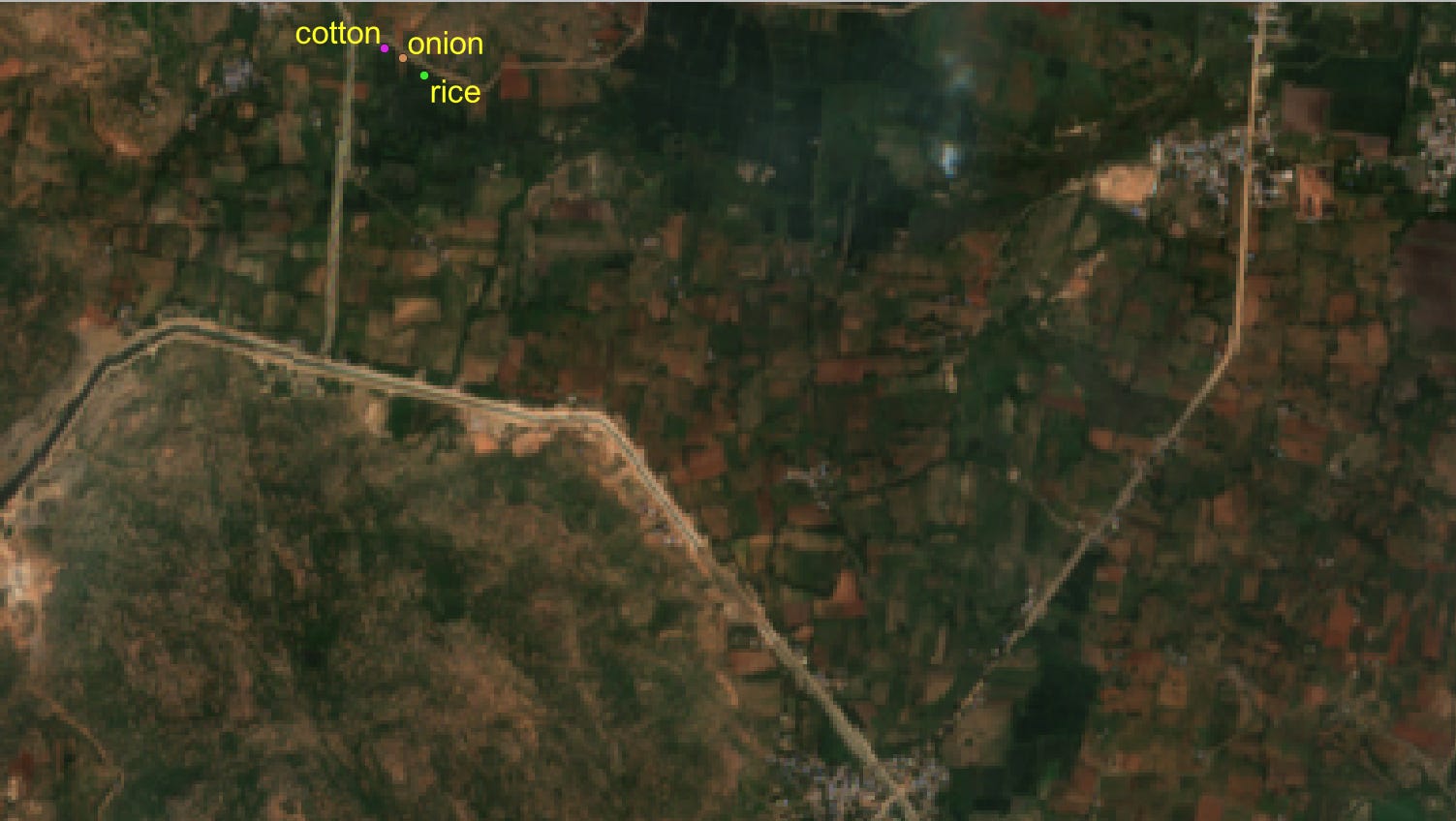
Let’s imagine we have a clear sky image which has already been labeled to indicate the presence of different crops, see Fig 1 below which is from the month of October , 2023 in Karnataka, India. You can notice the points of interest, the three fields where labeled data is available for crop grountruth in the same month as the clear image shown above.
With Satellite Cloud Generator we introduce varying degrees of cloudiness into the same image. The image below shows four SCG simulated images with increasing degrees of cloudiness derived from the same original image shown above.

Thick clouds such as the ones in the fourth image are very often caught by cloud masking algorithms, whereas thinner atmospheric clouds and haze as simulated in images 1,2 and 3 often go undetected. If we extract the RGB, NIR values for the pixels of the three crop groundtruth points we have and compute their respective NDVIs then we notice how the increased cloudiness adds some noise to the training data.
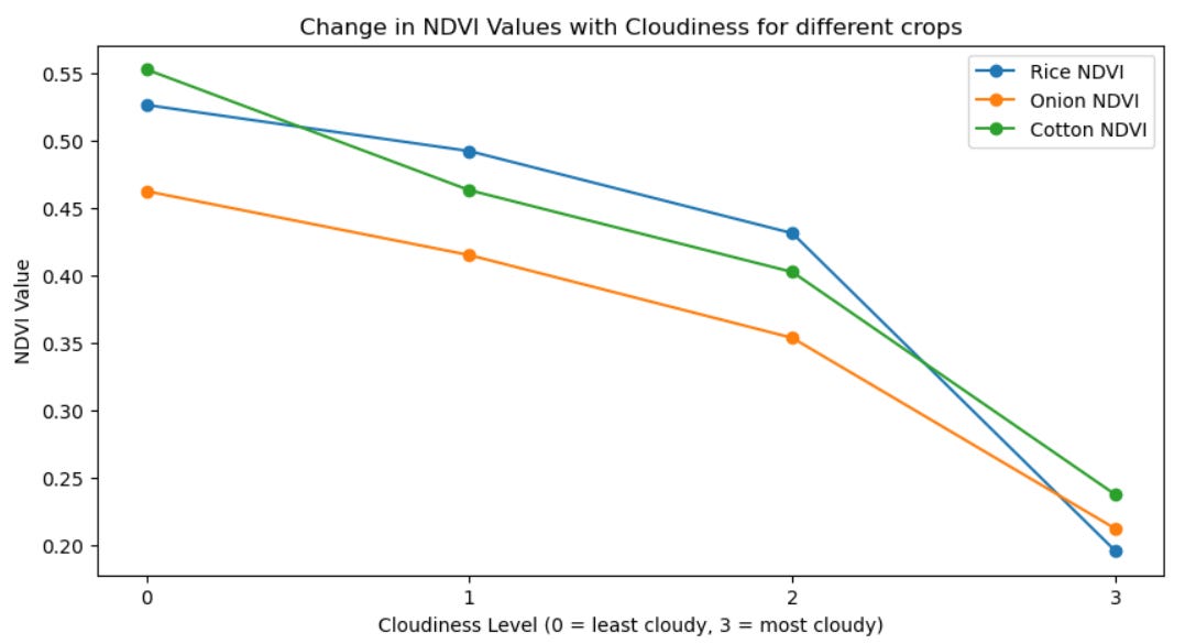
We can similarly add a predetermined cloudiness level to all images in a time series of images from an entire crop season and observe how this changes the relative patterns in the ndvi across the different crops.
As is the case with simulated data generally, the objective here is to add realistic noise to the original groundtruth in order to make the final model more robust to similar environmental noise it might see in real world conditions at inference. What do you think of these techniques, would they make sense in your workflows?